Chan–Vese:擬合邊界兩側的區域,找出輪廓
選讀・IP 11・影像分割(二):主動輪廓——蛇模型與水平集 的論文導讀(第 2/2 篇)。引用編號對應本頁底部的參考文獻。
導覽:本頁與本系列: 導覽:本頁與本系列
挑戰
只靠影像梯度驅動的輪廓,可能在模糊或微弱邊界失敗。Chan 與 Vese 的 TIP 2001 論文〈Active Contours Without Edges〉[8] 問的是:區域本身能否決定邊界?核心假設是兩個區域可用不同的常數強度作有效近似。「Without Edges」表示目標函數不需要邊緣偵測器,不代表輸出沒有邊界。閱讀數值推導前,先理解區域分割與水平集符號。
方法
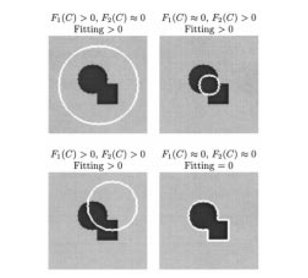
來源:Chan 與 Vese [8],TIP 2001,PDF 第 3 頁(印刷頁 268)、圖 1。原始 PDF。
以區域為基礎的輪廓能量為
是封閉輪廓, 是影像位置, 是觀測強度。 分別是目前內外區域的平均強度。非負 懲罰邊界長度, 是面積項權重,正值 加權兩種擬合誤差。積分在對應區域累積平方誤差。面積權重可以設為零,但比較有使用面積項的設定時,不能默默省略。
把原圖讀成能量論證。 輪廓落在暗物件內時,外部同時包含亮、暗像素,一個平均值難以擬合;輪廓落在物件外時,則換成內部混合。在理想分段常數範例中,對齊邊界可同時消除兩個擬合誤差。真實影像還須支付長度與面積成本,因此示意圖不代表所有真實邊界都能最小化完整能量。
以函數 的零水平集表示輪廓,採原論文的內部為正、外部為負慣例。正文採相反符號;切換慣例時,區域指示函數與演化式的符號也必須一致切換。演算法交替重新估計區域平均,並演化 以降低能量;階梯函數與 delta 函數的平滑近似讓數值演化可行。由於曲線是隱式表示,元件可自行分裂或合併,不必手動修改多邊形。最終分割仍受數值選擇、正規化與初始化影響。
結果
圖 4–6 展示含雜訊、模糊與細結構範例。圖 9 在平滑輪廓上比較此模型與使用邊緣函數的模型,後續範例則包含自然影像與沒有強梯度定義的輪廓。這些是區域擬合與拓樸處理機制的展示,不是資料集層級的分割準確度表格。報告的硬體時間也只屬於原實作及其影像尺寸。
消融與參數證據
論文研究階梯/delta 函數的正規化形式,並討論局部極小值。長度參數控制尺度:較大懲罰不利於小型或複雜輪廓,也可能把較小懲罰下分離的結構組在一起。這是參數與數值證據,不是現代的模組移除消融。除了最終遮罩,也要比較初始輪廓與停止條件;即使能量相同,改變初始化仍可能改變最佳化結果。
結論
此方法用區域統計的一致性,取代對強烈局部梯度的依賴。當物件與背景的平均強度可區分、邊界卻不明顯時,它很有用。先讀能量再讀求解器:更快的演化,無法補救不符合影像的區域模型。
限制與問題
照明變化、紋理或平均值相近的多個區域,可能違反雙常數假設。長度懲罰可能抹除小物件,而看似合理的遮罩未必是使用者想要的語意物件。能量非凸;示意圖與成功範例都不能證明從任意初始曲線全域收斂。加入其他區域模型或限制會改變方法,需要另外的證據。
參考文獻
- R. C. Gonzalez and R. E. Woods, Digital Image Processing, 4th ed., Pearson, 2018, Ch. 11. publisher page
- M. Kass, A. Witkin, and D. Terzopoulos, “Snakes: Active contour models,” International Journal of Computer Vision, vol. 1, no. 4, pp. 321–331, 1988. doi:10.1007/BF00133570
- C. Xu and J. L. Prince, “Snakes, shapes, and gradient vector flow,” IEEE Transactions on Image Processing, vol. 7, no. 3, pp. 359–369, 1998; see also C. Xu, A. Yezzi Jr., and J. L. Prince, “On the relationship between parametric and geometric active contours,” Proc. 34th Asilomar Conf. on Signals, Systems, and Computers, 2000. GVF project page with both papers
- L. D. Cohen, “On active contour models and balloons,” CVGIP: Image Understanding, vol. 53, no. 2, pp. 211–218, 1991. author PDF
- S. Osher and J. A. Sethian, “Fronts propagating with curvature-dependent speed: Algorithms based on Hamilton–Jacobi formulations,” Journal of Computational Physics, vol. 79, pp. 12–49, 1988. doi:10.1016/0021-9991(88)90002-2
- V. Caselles, R. Kimmel, and G. Sapiro, “Geodesic active contours,” International Journal of Computer Vision, vol. 22, no. 1, pp. 61–79, 1997. PDF
- D. Mumford and J. Shah, “Optimal approximations by piecewise smooth functions and associated variational problems,” Communications on Pure and Applied Mathematics, vol. 42, no. 5, pp. 577–685, 1989. doi:10.1002/cpa.3160420503
- T. F. Chan and L. A. Vese, “Active contours without edges,” IEEE Transactions on Image Processing, vol. 10, no. 2, pp. 266–277, 2001. doi:10.1109/83.902291
- D. Adalsteinsson and J. A. Sethian, “A fast level set method for propagating interfaces,” Journal of Computational Physics, vol. 118, pp. 269–277, 1995. summary page
- C. Li, C. Xu, C. Gui, and M. D. Fox, “Distance regularized level set evolution and its application to image segmentation,” IEEE Transactions on Image Processing, vol. 19, no. 12, pp. 3243–3254, 2010. doi:10.1109/TIP.2010.2069690
- P. Márquez-Neila, L. Baumela, and L. Álvarez, “A morphological approach to curvature-based evolution of curves and surfaces,” IEEE Transactions on Pattern Analysis and Machine Intelligence, 2014. doi:10.1109/TPAMI.2013.106
- scikit-image developers, “skimage.segmentation” API reference (
active_contour,chan_vese,morphological_chan_vese,morphological_geodesic_active_contour). docs - T. McInerney and D. Terzopoulos, “Deformable models in medical image analysis: A survey,” Medical Image Analysis, vol. 1, no. 2, 1996. author PDF
- D. Cremers, M. Rousson, and R. Deriche, “A review of statistical approaches to level set segmentation: Integrating color, texture, motion and shape,” International Journal of Computer Vision, vol. 72, no. 2, pp. 195–215, 2007. doi:10.1007/s11263-006-8711-1
- Y. Chen, P. Ge, G. Wang, and H. Chen, “An overview of intelligent image segmentation using active contour models,” Intelligence & Robotics, vol. 3, no. 1, pp. 23–55, 2023. open access
- S. Bohlender, I. Oksuz, and A. Mukhopadhyay, “A survey on shape-constraint deep learning for medical image segmentation,” IEEE Reviews in Biomedical Engineering, vol. 16, pp. 225–240, 2023. arXiv:2101.07721
- S. Peng, W. Jiang, H. Pi, X. Li, H. Bao, and X. Zhou, “Deep snake for real-time instance segmentation,” CVPR, 2020. arXiv:2001.01629
- X. Chen, B. M. Williams, S. R. Vallabhaneni, G. Czanner, R. Williams, and Y. Zheng, “Learning active contour models for medical image segmentation,” CVPR, 2019. CVF open access
- B. Kim and J. C. Ye, “Mumford–Shah loss functional for image segmentation with deep learning,” IEEE Transactions on Image Processing, vol. 29, pp. 1856–1866, 2020. doi · arXiv:1904.02872
- H. Kervadec, J. Bouchtiba, C. Desrosiers, E. Granger, J. Dolz, and I. Ben Ayed, “Boundary loss for highly unbalanced segmentation,” Medical Image Analysis, vol. 67, 2021 (first presented at MIDL 2019). arXiv:1812.07032