Chan–Vese: locate a boundary by fitting the regions on both sides
Optional · paper guide 2 of 2 for IP 11 · Image Segmentation II: Active Contours — Snakes and Level Sets. Citation numbers refer to the reference list at the bottom of this page.
Navigate: this page and this track: Navigate: this page and this track
Challenge
A contour driven only by image gradients can fail when the desired boundary is blurred or weak. Chan and Vese’s TIP 2001 paper, “Active Contours Without Edges” [8], asks whether the regions themselves can determine the boundary. Its central assumption is that two regions can be usefully approximated by different constant intensities. “Without edges” means that the objective does not need an edge detector; it does not mean the output has no boundary. Read region segmentation and level-set notation before the numerical derivation.
Method
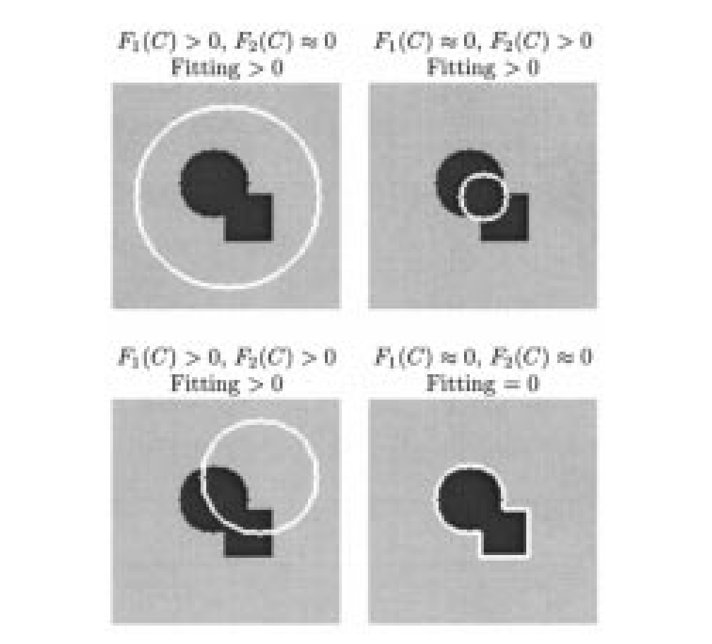
Source: Chan and Vese [8], TIP 2001, PDF page 3 (printed page 268), figure 1. Original PDF.
A region-based contour energy is
is the closed contour, an image position, and the observed intensity. are the mean intensities of the current inside and outside regions. Nonnegative penalizes boundary length, weights the area term, and positive weight the two fitting errors. The integrals accumulate squared errors over the respective regions. The area weight may be set to zero; it should not be silently omitted when comparing configurations that use it.
Follow the source diagram as an energy argument. When the contour lies inside the dark object, the outside contains both bright and dark pixels, which one mean fits poorly. When it lies outside the object, the inside becomes mixed instead. For the ideal piecewise-constant example, matching the boundary removes both fitting errors. Real images also pay length/area costs, so that cartoon does not prove every true boundary minimizes the complete energy.
Represent the contour as the zero level set of a function , using the paper’s convention of positive values inside and negative values outside. The main chapter uses the opposite sign; switching conventions requires switching the region indicators and evolution signs consistently. Alternate between recomputing the region means and evolving to reduce the energy. Smooth approximations to the step and delta functions make the numerical evolution possible. Because the curve is implicit, components can split or merge without explicitly editing a polygon. The final segmentation still depends on numerical choices, regularization and initialization.
Results
Figures 4–6 demonstrate noisy, blurred and thin-structure examples. Figure 9 compares the proposed model with an edge-function model on a smooth contour, while later examples include natural images and contours not defined by a strong gradient. These are demonstrations of the region-fitting mechanism and topology handling, not a dataset-wide segmentation accuracy table. The reported hardware timings also belong to the original implementation and image sizes.
Ablations and parameter evidence
The paper studies regularizations of the step/delta functions and discusses local minima. Its length parameter controls scale: a larger penalty discourages small or complicated contours and can group structures that remain separate with a smaller penalty. This is parameter and numerical evidence, not a modern module-removal ablation. Compare initial contours and stopping rules as well as final masks; changing the initialization can change the optimization outcome even when the energy is unchanged.
Conclusion
The method substitutes regional statistical agreement for a strong local gradient cue. It is useful when an object and background have distinguishable average intensities despite weak boundaries. Read the energy before the solver: a faster evolution cannot repair a region model that does not describe the image.
Problems
Illumination variation, texture or multiple regions with similar means can violate the two-constant assumption. A length penalty may erase small objects, and a plausible-looking mask need not correspond to the semantic object a user wants. The energy is nonconvex; neither the illustration nor successful examples establish global convergence from every starting curve. Additional region models or constraints change the method and require separate evidence.
References
- R. C. Gonzalez and R. E. Woods, Digital Image Processing, 4th ed., Pearson, 2018, Ch. 11. publisher page
- M. Kass, A. Witkin, and D. Terzopoulos, “Snakes: Active contour models,” International Journal of Computer Vision, vol. 1, no. 4, pp. 321–331, 1988. doi:10.1007/BF00133570
- C. Xu and J. L. Prince, “Snakes, shapes, and gradient vector flow,” IEEE Transactions on Image Processing, vol. 7, no. 3, pp. 359–369, 1998; see also C. Xu, A. Yezzi Jr., and J. L. Prince, “On the relationship between parametric and geometric active contours,” Proc. 34th Asilomar Conf. on Signals, Systems, and Computers, 2000. GVF project page with both papers
- L. D. Cohen, “On active contour models and balloons,” CVGIP: Image Understanding, vol. 53, no. 2, pp. 211–218, 1991. author PDF
- S. Osher and J. A. Sethian, “Fronts propagating with curvature-dependent speed: Algorithms based on Hamilton–Jacobi formulations,” Journal of Computational Physics, vol. 79, pp. 12–49, 1988. doi:10.1016/0021-9991(88)90002-2
- V. Caselles, R. Kimmel, and G. Sapiro, “Geodesic active contours,” International Journal of Computer Vision, vol. 22, no. 1, pp. 61–79, 1997. PDF
- D. Mumford and J. Shah, “Optimal approximations by piecewise smooth functions and associated variational problems,” Communications on Pure and Applied Mathematics, vol. 42, no. 5, pp. 577–685, 1989. doi:10.1002/cpa.3160420503
- T. F. Chan and L. A. Vese, “Active contours without edges,” IEEE Transactions on Image Processing, vol. 10, no. 2, pp. 266–277, 2001. doi:10.1109/83.902291
- D. Adalsteinsson and J. A. Sethian, “A fast level set method for propagating interfaces,” Journal of Computational Physics, vol. 118, pp. 269–277, 1995. summary page
- C. Li, C. Xu, C. Gui, and M. D. Fox, “Distance regularized level set evolution and its application to image segmentation,” IEEE Transactions on Image Processing, vol. 19, no. 12, pp. 3243–3254, 2010. doi:10.1109/TIP.2010.2069690
- P. Márquez-Neila, L. Baumela, and L. Álvarez, “A morphological approach to curvature-based evolution of curves and surfaces,” IEEE Transactions on Pattern Analysis and Machine Intelligence, 2014. doi:10.1109/TPAMI.2013.106
- scikit-image developers, “skimage.segmentation” API reference (
active_contour,chan_vese,morphological_chan_vese,morphological_geodesic_active_contour). docs - T. McInerney and D. Terzopoulos, “Deformable models in medical image analysis: A survey,” Medical Image Analysis, vol. 1, no. 2, 1996. author PDF
- D. Cremers, M. Rousson, and R. Deriche, “A review of statistical approaches to level set segmentation: Integrating color, texture, motion and shape,” International Journal of Computer Vision, vol. 72, no. 2, pp. 195–215, 2007. doi:10.1007/s11263-006-8711-1
- Y. Chen, P. Ge, G. Wang, and H. Chen, “An overview of intelligent image segmentation using active contour models,” Intelligence & Robotics, vol. 3, no. 1, pp. 23–55, 2023. open access
- S. Bohlender, I. Oksuz, and A. Mukhopadhyay, “A survey on shape-constraint deep learning for medical image segmentation,” IEEE Reviews in Biomedical Engineering, vol. 16, pp. 225–240, 2023. arXiv:2101.07721
- S. Peng, W. Jiang, H. Pi, X. Li, H. Bao, and X. Zhou, “Deep snake for real-time instance segmentation,” CVPR, 2020. arXiv:2001.01629
- X. Chen, B. M. Williams, S. R. Vallabhaneni, G. Czanner, R. Williams, and Y. Zheng, “Learning active contour models for medical image segmentation,” CVPR, 2019. CVF open access
- B. Kim and J. C. Ye, “Mumford–Shah loss functional for image segmentation with deep learning,” IEEE Transactions on Image Processing, vol. 29, pp. 1856–1866, 2020. doi · arXiv:1904.02872
- H. Kervadec, J. Bouchtiba, C. Desrosiers, E. Granger, J. Dolz, and I. Ben Ayed, “Boundary loss for highly unbalanced segmentation,” Medical Image Analysis, vol. 67, 2021 (first presented at MIDL 2019). arXiv:1812.07032