Guided Filter: fit local linear models instead of comparing every pair
Optional · paper guide 3 of 3 for IP 03 · Intensity Transformations and Spatial Filtering. Citation numbers refer to the reference list at the bottom of this page.
Navigate: this page and this track: Navigate: this page and this track
Challenge
He, Sun and Tang’s Guided Image Filtering paper [8] develops an edge-aware filter with an exact linear-time implementation in the number of pixels. This guide follows the expanded TPAMI 2013 paper, first presented at ECCV 2010. The goal is broader than denoising: use a guidance image to control the structure of a filtered signal. Know local means, variance and least squares before reading the derivation.
Method
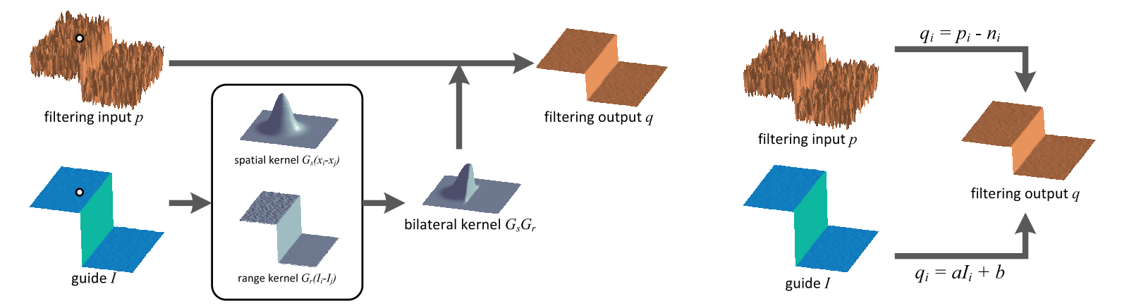
Source: He, Sun and Tang [8], TPAMI 2013 author PDF, page 3, figure 1. Original PDF.
In a window , assume the output is locally affine in scalar guidance : . Fit the coefficients to filtering input using
indexes a pixel, indexes a window, are its slope and offset, and penalizes a large slope. The overbars denote window means; covariance and variance also use that window. Average all overlapping predictions to obtain , where the last two means average coefficients of windows containing . Keeping only one window’s prediction would produce a different filter.
Follow the two inputs in the diagram. The guidance supplies the structural coordinate ; the input supplies the signal to approximate. When , the slope becomes local variance divided by variance plus : relatively flat regions are smoothed more, while strong local variation is more closely retained. With separate guidance, useful edges can transfer into the result—but so can irrelevant texture. For fixed guidance the output is linear in ; self-guided filtering is not globally linear because its coefficients depend on the input.
Algorithm 1 computes local statistics and coefficient averages using box filters. With constant-time box-sum updates per pixel, total cost is for pixels and does not grow with window radius in the same way as explicit pairwise evaluation. This is an implementation property of the stated algorithm, not a claim that every library implementation or color variant has identical runtime.
Results
The paper demonstrates smoothing, detail enhancement, structure transfer, matting/feathering, haze removal and joint upsampling. These are applications of the filter, not one common restoration benchmark. A particularly important reading trap is figure 2: its PSNR compares guided-filter outputs with bilateral-filter outputs. The bilateral result is not a clean ground truth, so that table measures agreement between filters rather than denoising accuracy.
Ablations and analytical evidence
The local-variance analysis explains how and window size affect smoothing. Figures 5–6 investigate gradient reversal when a base layer is subtracted and its detail residual amplified. The paper distinguishes the ideal local model from the final overlapping-window average; read its derivation and observed examples together rather than claiming an unconditional no-artifact theorem. Comparisons with a Gaussian-window variant further examine the shape of the effective kernel.
Conclusion
Choose this formulation when an aligned guidance image carries useful structure and efficient local filtering is the objective. It makes the distinction between “what to filter” and “what defines the edges” explicit. The chapter’s supplementary derivation supplies more algebra; this paper explains the algorithmic and experimental argument.
Problems
Misaligned guidance can move or duplicate boundaries. Guidance texture can imprint on a smoother target, and a noisy self-guidance image can retain unwanted variation. The regularizer has squared-intensity units, so changing the guidance scale requires changing . A filter used inside dehazing or depth upsampling does not independently validate the physical model or sensor calibration of the whole application.
References
- R. C. Gonzalez and R. E. Woods, Digital Image Processing, 4th ed., Pearson, 2018, Ch. 3. publisher page
- S. M. Pizer, E. P. Amburn, J. D. Austin, R. Cromartie, A. Geselowitz, T. Greer, B. ter Haar Romeny, J. B. Zimmerman and K. Zuiderveld, “Adaptive histogram equalization and its variations,” Computer Vision, Graphics, and Image Processing, 1987. doi
- K. Zuiderveld, “Contrast limited adaptive histogram equalization,” in P. S. Heckbert (ed.), Graphics Gems IV, Morgan Kaufmann, 1994, pp. 474–485. entry
- A. M. Reza, “Realization of the contrast limited adaptive histogram equalization (CLAHE) for real-time image enhancement,” Journal of VLSI Signal Processing, 2004. doi
- D. Coltuc, P. Bolon and J.-M. Chassery, “Exact histogram specification,” IEEE Transactions on Image Processing, 2006. doi
- C. Tomasi and R. Manduchi, “Bilateral filtering for gray and color images,” in Proc. IEEE International Conference on Computer Vision (ICCV), 1998. pdf
- S. Paris, P. Kornprobst, J. Tumblin and F. Durand, “Bilateral filtering: Theory and applications,” Foundations and Trends in Computer Graphics and Vision, vol. 4, no. 1, pp. 1–73, 2009. doi
- K. He, J. Sun and X. Tang, “Guided image filtering,” IEEE Transactions on Pattern Analysis and Machine Intelligence, 35(6):1397–1409, 2013 (first presented at ECCV 2010). doi
- P. Milanfar, “A tour of modern image filtering,” IEEE Signal Processing Magazine, vol. 30, no. 1, pp. 106–128, 2013. IEEE Xplore
- S. Gingichashvili and D. Lischinski, “Evaluation and comparison of edge-preserving filters,” arXiv:2012.13778, 2020. arXiv
- Y. Qi, Z. Yang, W. Sun et al., “A comprehensive overview of image enhancement techniques,” Archives of Computational Methods in Engineering, 2021. doi
- C. Li, C. Guo, L. Han, J. Jiang, M.-M. Cheng, J. Gu and C. C. Loy, “Low-light image and video enhancement using deep learning: A survey,” IEEE Transactions on Pattern Analysis and Machine Intelligence, 2021 (arXiv:2104.10729). arXiv
- C. Guo, C. Li, J. Guo, C. C. Loy, J. Hou, S. Kwong and R. Cong, “Zero-reference deep curve estimation for low-light image enhancement,” in Proc. IEEE/CVF CVPR, 2020. arXiv
- H. Zeng, J. Cai, L. Li, Z. Cao and L. Zhang, “Learning image-adaptive 3D lookup tables for high performance photo enhancement in real-time,” IEEE Transactions on Pattern Analysis and Machine Intelligence, 2020. arXiv
- M. Gharbi, J. Chen, J. T. Barron, S. W. Hasinoff and F. Durand, “Deep bilateral learning for real-time image enhancement,” ACM Transactions on Graphics (SIGGRAPH), 2017. arXiv
- H. Wu, S. Zheng, J. Zhang and K. Huang, “Fast end-to-end trainable guided filter,” in Proc. IEEE/CVF CVPR, 2018. arXiv
- Y. Cai, H. Bian, J. Lin, H. Wang, R. Timofte and Y. Zhang, “Retinexformer: One-stage Retinex-based transformer for low-light image enhancement,” in Proc. IEEE/CVF ICCV, 2023. arXiv
- S. Paris and F. Durand, “A fast approximation of the bilateral filter using a signal processing approach,” International Journal of Computer Vision, vol. 81, no. 1, pp. 24–52, 2009 (first presented at ECCV 2006). doi