U-Net:論文導讀
選讀・IP 10・影像分割(一):邊緣偵測、閾值化與區域偵測 的論文導讀(第 1/1 篇)。引用編號對應本頁底部的參考文獻。
導覽:本頁與本系列: 導覽:本頁與本系列
想像你要用手標記顯微鏡影像的每一個像素:一張就要花上數小時,所以一個實驗室可能只有幾十張標註好的影像。U-Net [14] 就是為這種情況設計的網路與訓練方法。這份補充資料說明論文宣稱了什麼、該怎麼讀它的結果;它是導讀,不是審查報告。
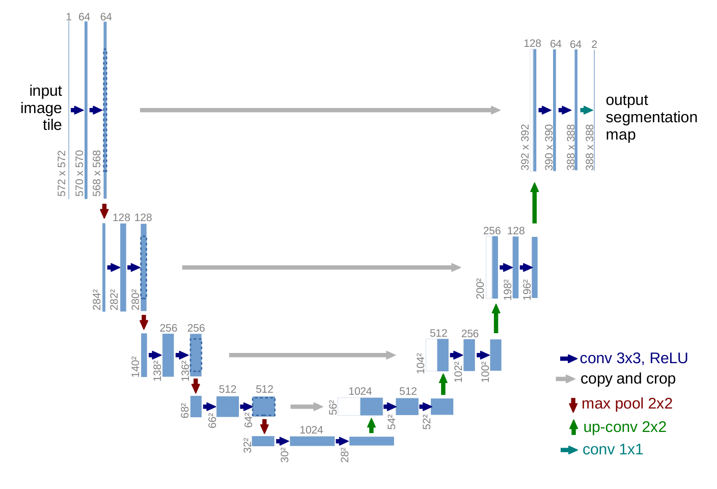
圖片來源: [14], arXiv:1505.04597v1, PDF 第 2 頁. 原始 PDF.
挑戰
生醫影像需要替每個像素指定類別,但已標註的影像很少。論文的出發點是較早的滑動視窗(sliding-window)網路:它用每個像素周圍的一塊小區域(patch)來分類該像素。作者指出兩個缺點:一是很慢,因為互相重疊的小區域會被反覆處理;二是定位與脈絡(context)互相取捨,較大的區域需要更多池化,會讓邊界變模糊。
方法
以全卷積網路(fully convolutional network)[13] 為基礎,並把它做成對稱的形狀。
- 收縮路徑(contracting path)重複「兩個 3×3 卷積加 ReLU,再接 2×2 最大池化」,每降一次取樣,通道數加倍。
- 擴張路徑(expanding path)先上取樣,再做一個把通道數減半的 2×2「上卷積」(up-convolution),接著與收縮路徑同一層、經裁切的特徵圖做串接(concatenation),最後做兩個 3×3 卷積。串接把精細的空間細節交給負責決定標籤的那幾層。論文本身沒有使用「跳接」(skip connection)一詞,圖中稱之為「copy and crop」。
- 所有卷積都不補邊(unpadded,也就是 “valid”),所以輸出比輸入小。大影像會被切成互相重疊的圖塊(overlap-tile 策略),影像邊緣缺少的脈絡以鏡射補齊。
縮小多少很容易算。每個 valid 的 3×3 卷積在每個維度減少 2 個像素,而且池化要求尺寸為偶數:
程式碼 · Python · 13 行
def unet_output_size(n, depth=4):
    """Output size of a U-Net with valid 3x3 convs, 2x2 pooling and 2x2 up-convs."""
    for _ in range(depth):          # contracting path
        n = n - 4                   # two valid 3x3 convs lose 2 pixels each
        assert n % 2 == 0, "max-pool needs an even size"
        n //= 2
    n = n - 4                       # bottom of the U: two valid convs
    for _ in range(depth):          # expanding path
        n = n * 2 - 4               # up-conv doubles, two valid convs lose 4
    return n

print(unet_output_size(572))                # 388
print((572 - unet_output_size(572)) // 2)   # 92
輸入 572×572 的圖塊(論文圖 1 所畫的尺寸)會得到 388×388 的輸出,所以圖塊每一側只提供了 92 個像素的脈絡。
替相接細胞設計的加權損失。 損失是逐像素的 softmax 交叉熵,再乘上權重圖 :
其中 是所有像素位置的集合, 是像素 處預測到真實類別 的機率, 用來平衡各類別出現的頻率,、 分別是 到最近與第二近細胞邊界的距離。指數項只在兩個細胞之間的細縫( 很小)才會很大。論文設定 、 像素(第 3 節)。論文印出的公式 (1) 沒有負號;上面的負號是「損失要最小化」時的慣用寫法。
彈性形變。 在粗略的 3×3 網格上,從標準差為 10 像素的高斯分布抽樣隨機位移向量,再以雙三次內插得到每個像素的位移(第 3.1 節)。作者說這「似乎是」用極少影像訓練分割網路的關鍵概念。
結果
第一個測試是 ISBI 2012 的電子顯微鏡(EM)神經結構分割挑戰賽 [21](30 張 512×512 像素的訓練影像),論文說該賽以 warping、Rand 與 pixel 三種誤差評分。在表 1(挑戰賽 2015 年 3 月 6 日的榜單快照,依 warping error 排序)中,U-Net(對 7 個旋轉版本的輸入取平均)的 warping error 為 0.000353,滑動視窗網路則是 0.000420。在表 2 中,針對細胞追蹤挑戰賽(cell tracking challenge)[22] 的兩個 2D 光學顯微鏡資料集,IOU 在 PhC-U373 上為 0.9203(35 張部分標註的訓練影像),在 DIC-HeLa 上為 0.7756(20 張),而 2015 年第二名分別是 0.83 與 0.46。訓練在單張 GPU 上約需 10 小時。
判讀證據
- 表 1 是排行榜,不是對照實驗。 測試標註是保密的,由主辦單位對提交的結果評分。U-Net 在 warping error 上只贏一點點:0.000353 對上第二名的 0.000355,論文沒有重複實驗或變異範圍。在 Rand error 上,表中有項目領先 U-Net,文中說明較好的那些方法對早期網路的機率圖做了高度針對該資料集的後處理;註腳寫著該演算法的作者提交了 78 組不同的解。請確認標題數字用的是哪個指標,以及「第一名」到底值多少。
- 對 7 個旋轉輸入取平均屬於測試時擴增(test-time augmentation)。 要問比較對象是否也享有同樣待遇。
- 表 2 的來源不一。 競爭者的數字來自挑戰賽,不是作者重跑的結果,而「2015 年第二名」只寫到兩位小數。論文沒有說明競爭的參賽者是否使用相同的訓練影像。
限制與問題
論文沒有任何消融實驗(ablation):沒有把加權損失、彈性形變或串接拿掉來量測各自的效果,所以那句「關鍵概念」是作者的看法,不是實驗結果。三個資料集都是小型 2D 顯微鏡資料,也沒有報告重複實驗或變異。這套做法在其他類型的影像或 3D 上是否有效,論文並未測試。
結論
在本教學中,U-Net 是兩個傳統想法的學習版對應:多尺度分析(收縮路徑),以及利用精細資料精確定位邊界(串接進來的高解析度特徵)。這種「編碼器–解碼器加上同層連接」的結構,後來成為分割以外的常見骨幹;影像修復的部分,請見 DLCV 04・深度影像復原。
參考文獻
- R. C. Gonzalez and R. E. Woods, Digital Image Processing, 4th ed., Pearson, 2018, Ch. 10. publisher page
- D. Marr and E. Hildreth, “Theory of edge detection,” Proceedings of the Royal Society of London. Series B, vol. 207, no. 1167, pp. 187–217, 1980. doi
- J. Canny, “A Computational Approach to Edge Detection,” IEEE Transactions on Pattern Analysis and Machine Intelligence, vol. PAMI-8, no. 6, pp. 679–698, 1986. doi
- R. O. Duda and P. E. Hart, “Use of the Hough transformation to detect lines and curves in pictures,” Communications of the ACM, vol. 15, pp. 11–15, 1972. doi
- N. Otsu, “A Threshold Selection Method from Gray-Level Histograms,” IEEE Transactions on Systems, Man, and Cybernetics, vol. 9, no. 1, pp. 62–66, 1979. doi
- M. Sezgin and B. Sankur, “Survey over image thresholding techniques and quantitative performance evaluation,” Journal of Electronic Imaging, vol. 13, no. 1, pp. 146–165, 2004. doi
- J. Sauvola and M. Pietikäinen, “Adaptive document image binarization,” Pattern Recognition, vol. 33, no. 2, pp. 225–236, 2000. doi
- R. Achanta, A. Shaji, K. Smith, A. Lucchi, P. Fua and S. Süsstrunk, “SLIC Superpixels Compared to State-of-the-Art Superpixel Methods,” IEEE Transactions on Pattern Analysis and Machine Intelligence, vol. 34, no. 11, pp. 2274–2282, 2012. doi
- J. Shi and J. Malik, “Normalized cuts and image segmentation,” IEEE Transactions on Pattern Analysis and Machine Intelligence, vol. 22, no. 8, pp. 888–905, 2000. doi
- L. Vincent and P. Soille, “Watersheds in digital spaces: an efficient algorithm based on immersion simulations,” IEEE Transactions on Pattern Analysis and Machine Intelligence, vol. 13, no. 6, pp. 583–598, 1991. doi
- S. Minaee, Y. Boykov, F. Porikli, A. Plaza, N. Kehtarnavaz and D. Terzopoulos, “Image Segmentation Using Deep Learning: A Survey,” IEEE Transactions on Pattern Analysis and Machine Intelligence, vol. 44, no. 7, pp. 3523–3542, 2022. doi · arXiv
- T. Zhou, W. Xia, F. Zhang, B. Chang, W. Wang, Y. Yuan, E. Konukoglu and D. Cremers, “Image Segmentation in Foundation Model Era: A Survey,” arXiv:2408.12957, 2024. arXiv
- J. Long, E. Shelhamer and T. Darrell, “Fully Convolutional Networks for Semantic Segmentation,” arXiv:1411.4038, 2014. arXiv
- O. Ronneberger, P. Fischer and T. Brox, “U-Net: Convolutional Networks for Biomedical Image Segmentation,” in Medical Image Computing and Computer-Assisted Intervention – MICCAI 2015, Lecture Notes in Computer Science, vol. 9351, pp. 234–241, Springer, 2015. doi · arXiv
- K. He, G. Gkioxari, P. Dollár and R. Girshick, “Mask R-CNN,” arXiv:1703.06870, 2017. arXiv
- L.-C. Chen, G. Papandreou, I. Kokkinos, K. Murphy and A. L. Yuille, “DeepLab: Semantic Image Segmentation with Deep Convolutional Nets, Atrous Convolution, and Fully Connected CRFs,” IEEE Transactions on Pattern Analysis and Machine Intelligence, vol. 40, no. 4, pp. 834–848, 2018. doi · arXiv
- A. Kirillov, E. Mintun, N. Ravi et al., “Segment Anything,” arXiv:2304.02643, 2023. arXiv
- R. Sun, T. Lei, Q. Chen, Z. Wang, X. Du, W. Zhao and A. K. Nandi, “Survey of Image Edge Detection,” Frontiers in Signal Processing, 2022. doi
- S. Xie and Z. Tu, “Holistically-Nested Edge Detection,” arXiv:1504.06375, 2015. arXiv
- D. Stutz, A. Hermans and B. Leibe, “Superpixels: An Evaluation of the State-of-the-Art,” Computer Vision and Image Understanding, vol. 166, pp. 1–27, 2018. doi
- I. Arganda-Carreras, S. C. Turaga, D. R. Berger et al., “Crowdsourcing the creation of image segmentation algorithms for connectomics,” Frontiers in Neuroanatomy, vol. 9, 2015. doi
- M. Maška, V. Ulman, D. Svoboda et al., “A benchmark for comparison of cell tracking algorithms,” Bioinformatics, vol. 30, no. 11, pp. 1609–1617, 2014. doi · Cell Tracking Challenge