形態學的理論基礎
選讀・IP 09・形態學影像處理 的論文導讀(第 1/1 篇)。引用編號對應本頁底部的參考文獻。
導覽:本頁與本系列: 導覽:本頁與本系列
論點
Matheron 的隨機集合 [2]、Serra 的數學形態學 [3]、Haralick、Sternberg 與 Zhuang 的工程教學 [4],以及 Soille 的實作參考書 [5],把形狀運算連到代數。重點不只是收集「變粗、變細」濾波器,而是以定義保證包含、順序與重複運算的性質,協助組合演算法。
運算與假設
對前景集合 與結構元素 ,採用:
是膨脹, 是侵蝕, 為平移後結構元素。 的原點、方向都是定義一部分;若不對稱,補集/對偶公式必須注意反射,比較實作前也須確認函式庫慣例。
斷開為 ,閉合為 ,兩階段使用相同 。斷開保留能容納平移結構元素的部分,閉合填入部分可被結構元素跨越的間隙;兩者都不是推估退化前的真實物體。
具體範例
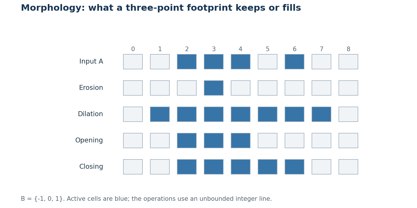
取一維集合 、。侵蝕剩 ,膨脹為 ,斷開為 ,閉合為 。斷開移除位置 6 的孤立點,閉合填入位置 5 的間隙。配圖是教材自行計算的例子,不是原書/論文實驗結果。
結果依賴 的尺度、形狀,更換結構元素會保留或移除不同特徵。實際影像還要考慮前景連通性與邊界填補,才能知道靠邊位置的運算意義。
如何閱讀理論
定義須與假設、證明一起讀。斷開具有遞增、反廣延及冪等性:較大輸入的斷開不會小於較小輸入的斷開,斷開包含於輸入,重做同一斷開不再改變結果。閉合則具有對應的廣延與冪等性。這說明何時重複運算多餘,也說明更換結構元素是另一種介入。
基礎文獻建立集合/格理論觀點,Haralick 等人連接二值、灰階定義與演算法,Soille 再涵蓋重建、測地運算、分水嶺與效率。灰階鄰域最大/最小是順序上的擴充,不是把二值集合公式直接逐通道套到任意 RGB 色彩。
結論
明確指定結構元素、原點與代數性質,才能推理形態學行為。這些書籍、教學提供互補的數學與實作觀點,不是互相比拚測試分數的模型。
限制
結構元素編入幾何假設,可能移除有效細線或合併不同物體。邊界慣例會使表面相似的實作不同,理論冪等性也假設運算定義完全相同。它們不提供學習式語意理解,也不保證改過的遮罩更準確;仍須對應應用的證據。
參考文獻
- R. C. Gonzalez and R. E. Woods, Digital Image Processing, 4th ed., Pearson, 2018, Ch. 9. publisher page
- G. Matheron, Random Sets and Integral Geometry, Wiley, 1975. library record
- J. Serra, Image Analysis and Mathematical Morphology, Academic Press, 1982. library record
- R. M. Haralick, S. R. Sternberg, and X. Zhuang, “Image Analysis Using Mathematical Morphology,” IEEE Trans. Pattern Analysis and Machine Intelligence, vol. PAMI-9, pp. 532–550, 1987. doi
- P. Soille, Morphological Image Analysis, Springer, 2004. doi
- T. Y. Zhang and C. Y. Suen, “A Fast Parallel Algorithm for Thinning Digital Patterns,” Communications of the ACM, vol. 27, pp. 236–239, 1984. doi
- L. Vincent, “Morphological Grayscale Reconstruction in Image Analysis: Applications and Efficient Algorithms,” IEEE Trans. Image Processing, vol. 2, pp. 176–201, 1993. doi
- P. Maragos, “Pattern Spectrum and Multiscale Shape Representation,” IEEE Trans. Pattern Analysis and Machine Intelligence, vol. 11, no. 7, pp. 701–716, 1989. doi
- E. J. Breen and R. Jones, “Attribute Openings, Thinnings, and Granulometries,” Computer Vision and Image Understanding, vol. 64, no. 3, pp. 377–389, 1996. doi
- P. Salembier and M. H. F. Wilkinson, “Connected Operators: A Review of Region-Based Morphological Image Processing Techniques,” IEEE Signal Processing Magazine, vol. 26, no. 6, pp. 136–157, 2009. doi
- E. Carlinet and T. Géraud, “A Comparative Review of Component Tree Computation Algorithms,” IEEE Trans. Image Processing, vol. 23, pp. 3885–3895, 2014. doi
- S. van der Walt et al., “scikit-image: Image Processing in Python,” PeerJ, 2014. arXiv
- R. Mondal, S. Santra, S. S. Mukherjee, and B. Chanda, “Morphological Network: How Far Can We Go with Morphological Neurons?,” BMVC, 2022. arXiv
- K. Nogueira, J. Chanussot, M. Dalla Mura, and J. A. dos Santos, “An Introduction to Deep Morphological Networks,” arXiv:1906.01751, 2019. arXiv
- R. Hermary, G. Tochon, É. Puybareau, A. Kirszenberg, and J. Angulo, “Learning Grayscale Mathematical Morphology with Smooth Morphological Layers,” Journal of Mathematical Imaging and Vision, vol. 64, pp. 736–753, 2022. doi
- A. Kirszenberg, G. Tochon, É. Puybareau, and J. Angulo, “Going Beyond p-convolutions to Learn Grayscale Morphological Operators,” arXiv:2102.10038, 2021. arXiv
- S. Shit et al., “clDice — A Novel Topology-Preserving Loss Function for Tubular Structure Segmentation,” CVPR, 2021. arXiv