Foundations of mathematical morphology
Optional · paper guide 1 of 1 for IP 09 · Morphological Image Processing. Citation numbers refer to the reference list at the bottom of this page.
Navigate: this page and this track: Navigate: this page and this track
The argument
Matheron’s random-set treatment [2], Serra’s mathematical morphology [3], the engineering tutorial by Haralick, Sternberg and Zhuang [4], and Soille’s practical reference [5] connect shape operations to an algebra. The point is not merely to collect filters that make objects thicker or thinner: definitions give predictable inclusion, order and repetition properties that help compose an algorithm.
Operators and assumptions
For a foreground set and a structuring set , use
is dilation, erosion, and is a translated structuring set. The origin and orientation of are part of the definition. Reflection matters in complement/duality formulas when is not symmetric; library conventions must be checked before comparing implementations.
Opening is ; closing is . The same is used in both stages. Opening keeps the parts that can accommodate translated copies of the structuring set. Closing fills some gaps that the structuring set bridges. Neither operator infers the true object that existed before corruption.
Worked evidence
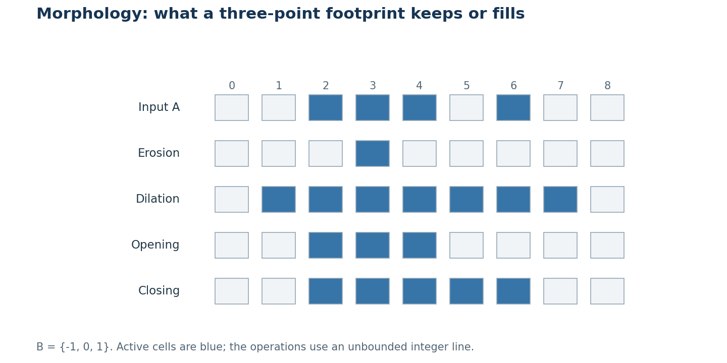
Use the one-dimensional example and . Erosion leaves , dilation gives , opening gives , and closing gives . The isolated point at 6 disappears under opening; the gap at 5 fills under closing. The figure is an original worked example, not an experimental result from these books/papers.
These outcomes depend on the scale and shape of . A different structuring set can preserve or remove a different feature. In images, foreground connectivity and boundary padding also determine what the operation means near an edge.
How to read the theory
Read an operator definition together with its hypotheses and proven properties. Opening is increasing, anti-extensive and idempotent: enlarging an input cannot shrink its opening relative to a smaller input, the opening lies inside its input, and applying the same opening twice changes nothing. Closing has the corresponding extensive and idempotent behavior. This explains when repeating an operation is redundant and why changing its footprint is a different intervention.
The foundational sources establish set/lattice reasoning. Haralick et al. connect binary and grayscale definitions to algorithms; Soille expands toward reconstruction, geodesic operations, watersheds and efficient implementations. A grayscale max/min neighborhood is an order-based extension, not simply the binary set formula applied independently to arbitrary RGB colors.
Conclusion
Morphology becomes easier to reason about when a chosen footprint, its origin and the algebraic properties are explicit. The books and tutorial provide complementary mathematical and implementation viewpoints rather than competing benchmark models.
Limits
The footprint encodes a geometric assumption and may erase legitimate thin structures or merge separate objects. Border conventions can invalidate a naive comparison, and theoretical idempotence assumes the same precisely defined operator. These sources do not supply learned semantic understanding or guarantee that a changed mask is more accurate for a particular application; that requires task-specific evidence.
References
- R. C. Gonzalez and R. E. Woods, Digital Image Processing, 4th ed., Pearson, 2018, Ch. 9. publisher page
- G. Matheron, Random Sets and Integral Geometry, Wiley, 1975. library record
- J. Serra, Image Analysis and Mathematical Morphology, Academic Press, 1982. library record
- R. M. Haralick, S. R. Sternberg, and X. Zhuang, “Image Analysis Using Mathematical Morphology,” IEEE Trans. Pattern Analysis and Machine Intelligence, vol. PAMI-9, pp. 532–550, 1987. doi
- P. Soille, Morphological Image Analysis, Springer, 2004. doi
- T. Y. Zhang and C. Y. Suen, “A Fast Parallel Algorithm for Thinning Digital Patterns,” Communications of the ACM, vol. 27, pp. 236–239, 1984. doi
- L. Vincent, “Morphological Grayscale Reconstruction in Image Analysis: Applications and Efficient Algorithms,” IEEE Trans. Image Processing, vol. 2, pp. 176–201, 1993. doi
- P. Maragos, “Pattern Spectrum and Multiscale Shape Representation,” IEEE Trans. Pattern Analysis and Machine Intelligence, vol. 11, no. 7, pp. 701–716, 1989. doi
- E. J. Breen and R. Jones, “Attribute Openings, Thinnings, and Granulometries,” Computer Vision and Image Understanding, vol. 64, no. 3, pp. 377–389, 1996. doi
- P. Salembier and M. H. F. Wilkinson, “Connected Operators: A Review of Region-Based Morphological Image Processing Techniques,” IEEE Signal Processing Magazine, vol. 26, no. 6, pp. 136–157, 2009. doi
- E. Carlinet and T. Géraud, “A Comparative Review of Component Tree Computation Algorithms,” IEEE Trans. Image Processing, vol. 23, pp. 3885–3895, 2014. doi
- S. van der Walt et al., “scikit-image: Image Processing in Python,” PeerJ, 2014. arXiv
- R. Mondal, S. Santra, S. S. Mukherjee, and B. Chanda, “Morphological Network: How Far Can We Go with Morphological Neurons?,” BMVC, 2022. arXiv
- K. Nogueira, J. Chanussot, M. Dalla Mura, and J. A. dos Santos, “An Introduction to Deep Morphological Networks,” arXiv:1906.01751, 2019. arXiv
- R. Hermary, G. Tochon, É. Puybareau, A. Kirszenberg, and J. Angulo, “Learning Grayscale Mathematical Morphology with Smooth Morphological Layers,” Journal of Mathematical Imaging and Vision, vol. 64, pp. 736–753, 2022. doi
- A. Kirszenberg, G. Tochon, É. Puybareau, and J. Angulo, “Going Beyond p-convolutions to Learn Grayscale Morphological Operators,” arXiv:2102.10038, 2021. arXiv
- S. Shit et al., “clDice — A Novel Topology-Preserving Loss Function for Tubular Structure Segmentation,” CVPR, 2021. arXiv