Non-Local Means: use similar patches to decide which pixels to average
Optional · paper guide 2 of 3 for IP 05 · Image Restoration and Reconstruction. Citation numbers refer to the reference list at the bottom of this page.
Navigate: this page and this track: Navigate: this page and this track
Challenge
Nearby pixels are not necessarily samples of the same underlying signal. A repeated window or stripe farther away may be more useful for denoising than a pixel across a nearby boundary. Non-Local Means (NLM) introduced patch similarity as a way to find such evidence [7]. This guide follows Buades, Coll and Morel’s reproducible IPOL 2011 article, “Non-Local Means Denoising” [23], including its noise correction and patchwise implementation; these details should not be silently attributed to every implementation of the original CVPR 2005 method.
Method
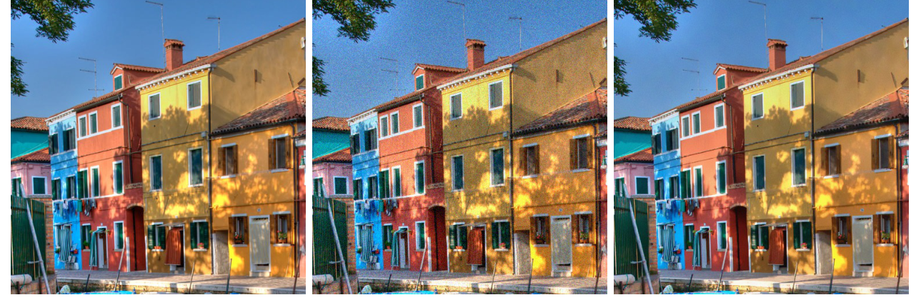
Source: Buades, Coll and Morel [23], IPOL 2011, PDF page 4, figure 1; current PDF dated 2015/06/16. Original PDF. Source photograph credited to Hervé Bry, CC BY-NC-SA, as recorded in the paper. The paper provides a result figure rather than an architecture diagram.
For a scalar noisy image, the pixelwise estimator and the IPOL weight are
is the noisy intensity at candidate center , is the search window around target , are equal-sized patches, and is their mean squared difference. The noise standard deviation is and controls averaging strength. For color, distance also averages over channels and the same weights are used for each output channel.
Why subtract noise energy? Under independent, equal-variance additive noise, the expected squared difference between two noisy samples contains a contribution. The correction avoids treating all of that difference as genuine signal mismatch. It is a statistical correction, not knowledge of which particular pixels are noisy. The IPOL implementation also replaces the self-weight by the largest other candidate weight so that the reference pixel does not automatically dominate.
Separate comparison from aggregation. Pixelwise NLM uses a patch to choose weights but estimates only its center. Patchwise NLM uses those weights to estimate the entire reference patch, then averages the overlapping patch predictions at each output pixel. Neither version trains a dataset-level model. “Non-local” also does not require searching the whole image: the documented implementation restricts the search to a larger local window for computational reasons.
Results
Figure 1 shows a color example with added noise at . It demonstrates removal of visible noise while retaining structures; one visual example is not a comprehensive robustness benchmark. Table 1 specifies reproducible parameter settings: for grayscale , it uses a comparison patch, a search window and . These parameters use the article’s intensity scale. Normalizing intensities requires scaling both and .
Ablations and implementation evidence
Section 3 compares pixelwise and patchwise formulations. The authors report a PSNR benefit and reduced spurious edge oscillations from final patch aggregation, while explicitly stating that overall detail preservation is not improved. This is an implementation comparison, not a table proving that larger patches always win. The parameter schedule increases patch and search sizes as noise grows; robustness of similarity estimates and availability of matches are separate concerns.
Conclusion
NLM turns denoising into finding repeated local structure and averaging compatible evidence. Use it as a transparent, training-free baseline when self-similarity and the noise assumptions are reasonable. Read BM3D next: it also groups similar patches, but jointly transforms and shrinks the group instead of relying only on weighted averaging.
Problems
Unique details may lack suitable matches; repeated textures with different phases can be confused. Strong noise corrupts the distance used to select evidence, and correlated or signal-dependent noise breaks the simple correction’s assumptions. Large searches cost more and may admit misleading candidates. Patch aggregation reuses overlapping observations, so its predictions should not be treated as independent samples when reasoning about uncertainty.
References
- R. C. Gonzalez and R. E. Woods, Digital Image Processing, 4th ed., Pearson, 2018, Ch. 5. publisher page
- H. Hwang and R. A. Haddad, “Adaptive median filters: new algorithms and results,” IEEE Transactions on Image Processing, vol. 4, no. 4, pp. 499–502, 1995. DOI
- B. R. Hunt, “The application of constrained least squares estimation to image restoration by digital computer,” IEEE Transactions on Computers, vol. C-22, no. 9, pp. 805–812, 1973. DOI
- A. C. Kak and M. Slaney, Principles of Computerized Tomographic Imaging, IEEE Press, 1988 (SIAM reprint 2001). free online edition
- L. A. Shepp and B. F. Logan, “The Fourier reconstruction of a head section,” IEEE Transactions on Nuclear Science, vol. 21, no. 3, pp. 21–43, 1974. DOI
- scikit-image developers, “Radon transform,” scikit-image documentation (gallery example). docs
- A. Buades, B. Coll and J.-M. Morel, “A non-local algorithm for image denoising,” IEEE CVPR, vol. 2, pp. 60–65, 2005. DOI
- K. Dabov, A. Foi, V. Katkovnik and K. Egiazarian, “Image denoising by sparse 3-D transform-domain collaborative filtering,” IEEE Transactions on Image Processing, vol. 16, no. 8, pp. 2080–2095, 2007. DOI
- K. Zhang, W. Zuo, Y. Chen, D. Meng and L. Zhang, “Beyond a Gaussian denoiser: Residual learning of deep CNN for image denoising,” IEEE Transactions on Image Processing, vol. 26, no. 7, pp. 3142–3155, 2017. doi · arXiv
- C. Tian, L. Fei, W. Zheng, Y. Xu, W. Zuo and C.-W. Lin, “Deep learning on image denoising: An overview,” Neural Networks, vol. 131, pp. 251–275, 2020. arXiv
- M. Elad, B. Kawar and G. Vaksman, “Image denoising: The deep learning revolution and beyond — A survey paper,” SIAM Journal on Imaging Sciences, vol. 16, no. 3, pp. 1594–1654, 2023. arXiv
- K. Zhang, W. Ren, W. Luo, W.-S. Lai, B. Stenger, M.-H. Yang and H. Li, “Deep image deblurring: A survey,” International Journal of Computer Vision, 2022. arXiv
- G. Ongie, A. Jalal, C. A. Metzler, R. G. Baraniuk, A. G. Dimakis and R. Willett, “Deep learning techniques for inverse problems in imaging,” arXiv:2005.06001, 2020. arXiv
- U. S. Kamilov, C. A. Bouman, G. T. Buzzard and B. Wohlberg, “Plug-and-play methods for integrating physical and learned models in computational imaging: Theory, algorithms, and applications,” IEEE Signal Processing Magazine, vol. 40, no. 1, pp. 85–97, 2023. arXiv
- K. Zhang, Y. Li, W. Zuo, L. Zhang, L. Van Gool and R. Timofte, “Plug-and-play image restoration with deep denoiser prior,” IEEE Transactions on Pattern Analysis and Machine Intelligence, vol. 44, no. 10, pp. 6360–6376, 2022. arXiv
- K. H. Jin, M. T. McCann, E. Froustey and M. Unser, “Deep convolutional neural network for inverse problems in imaging,” IEEE Transactions on Image Processing, vol. 26, no. 9, pp. 4509–4522, 2017. arXiv
- J. Adler and O. Öktem, “Learned primal-dual reconstruction,” IEEE Transactions on Medical Imaging, 2018. arXiv
- V. Monga, Y. Li and Y. C. Eldar, “Algorithm unrolling: Interpretable, efficient deep learning for signal and image processing,” arXiv:1912.10557, 2019. arXiv
- G. Wang, J. C. Ye and B. De Man, “Deep learning for tomographic image reconstruction,” Nature Machine Intelligence, vol. 2, no. 12, pp. 737–748, 2020. DOI
- A. Buades, B. Coll and J.-M. Morel, “A review of image denoising algorithms, with a new one,” Multiscale Modeling & Simulation, vol. 4, no. 2, pp. 490–530, 2005. DOI
- L. I. Rudin, S. Osher and E. Fatemi, “Nonlinear total variation based noise removal algorithms,” Physica D: Nonlinear Phenomena, vol. 60, no. 1–4, pp. 259–268, 1992. DOI
- A. Chambolle, “An algorithm for total variation minimization and applications,” Journal of Mathematical Imaging and Vision, vol. 20, no. 1–2, pp. 89–97, 2004. DOI
- A. Buades, B. Coll and J.-M. Morel, “Non-Local Means Denoising,” Image Processing On Line, vol. 1, pp. 208–212, 2011. DOI · article and implementation