The reviews in more detail
Optional · paper guide 1 of 1 for IP 02 · Digital Image Fundamentals. Citation numbers refer to the reference list at the bottom of this page.
Navigate: this page and this track: Navigate: this page and this track
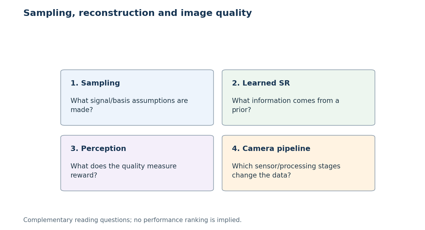
Choose a reading by topic: Sampling, Learned SR, Perception, Camera pipeline.
Sampling and interpolation theory
Unser’s “Sampling — 50 years after Shannon” [2] reframes sampling as approximation in shift-invariant spaces: instead of demanding a perfectly band-limited signal and an ideal sinc reconstructor, choose a practical basis (such as B-splines) and project onto it. Its main takeaway is to analyze the sampling basis, prefilter and reconstruction kernel together; none removes the information limit imposed by the sampling rate. Thévenaz, Blu and Unser [4] apply this to image interpolation and compare many kernels on equal terms. They show that approximation order and kernel support explain most of the differences, and that B-spline-based interpolation (with a proper prefilter) offers a better quality-for-cost trade-off than Keys’ cubic convolution [3]. Both papers remain the reference point for anyone who implements resizing.
Learned super-resolution
Wang, Chen and Hoi [9] survey deep super-resolution up to about 2019: network designs, upsampling layers placed early or late, loss functions, and benchmarks. Moser et al. [10] extend the picture to transformers and diffusion models and stress open problems such as flexible scale factors and better evaluation. Two works show how the classical ideas survive inside networks. LIIF [11] represents an image as a continuous function queried at any coordinate — a learned interpolator that can upsample by arbitrary factors, including factors not seen in training. Real-ESRGAN [12] tackles the gap between the bicubic downsampling used to create most training pairs and real degradations, by synthesizing training data with a higher-order degradation model that applies blur, noise, resizing and compression more than once. The lesson for this chapter: bicubic interpolation is both the baseline every method is compared against and, through its use in creating training data, a hidden assumption that can make models fail on real images.
Perception and image quality
Wang et al.’s SSIM [13] turned the observations of the perception section — sensitivity to structure and relative change rather than absolute error — into a full-reference quality index that compares local luminance, contrast and structure. Zhai and Min [14] survey the whole field of perceptual quality assessment: full-, reduced- and no-reference methods, and models for specialized content. Deep features changed this area markedly. Zhang et al. [15] collected human similarity judgments and found that distances between deep network features (LPIPS) agree better with the collected human judgments than the compared traditional metrics under their benchmark, with transfer across the tested architectures and training regimes. Ding et al. [16] then asked a sharper question: if you optimize an image-processing network with each quality metric as the loss, which metric gives results people prefer? Their human study shows that rankings on standard quality benchmarks do not reliably predict usefulness as a training objective. In short, Mach bands and the Weber ratio now live inside loss functions.
Camera sensor pipelines
Ramanath et al. [8] describe the classic in-camera pipeline that sits between the sensor array of this chapter and the compressed file you save: demosaicking, white balance, color transforms, gamma, and compression, each a fixed hand-designed stage. Delbracio et al. [7] tour how mobile computational photography reworked this pipeline over two decades, with burst capture, alignment and merging (the averaging-noisy-images idea at scale), and multi-frame super-resolution. Learned replacements now exist for parts or all of it. Chen et al. [17] trained a network to map raw short-exposure sensor data directly to a clean image in very low light, bypassing the traditional pipeline. Ignatov et al. [18] replaced an entire smartphone image signal processor with one network (PyNET) trained to map raw mosaic sensor data to images resembling those from a DSLR.
Reading these papers critically
Read these sources as answers to different questions. The sampling papers specify which continuous-signal model and reconstruction basis justify an interpolator; the learned-SR papers add a data-dependent prior; the quality papers evaluate the resulting image; and the camera-pipeline papers explain how the observations were produced. Those roles are complementary, not a ranking of algorithms that solve the same problem. In particular, interpolation quality cannot be compared fairly without fixing the downsampling filter, boundary handling and output coordinates.
For an empirical comparison, distinguish a reference-image error from a perceptual judgment and from a downstream task score. A learned model may look sharper by inventing plausible detail, while a sensor-domain method can exploit information absent from a finished RGB file. Read each result under its available inputs and evaluation protocol. The practical next step is to state the image-formation assumptions first, then choose reconstruction and evaluation that answer the intended question.
References
- R. C. Gonzalez and R. E. Woods, Digital Image Processing, 4th ed., Pearson, 2018, Ch. 2. publisher page
- M. Unser, “Sampling—50 years after Shannon,” Proceedings of the IEEE, vol. 88, no. 4, pp. 569–587, 2000. doi
- R. Keys, “Cubic convolution interpolation for digital image processing,” IEEE Transactions on Acoustics, Speech, and Signal Processing, vol. 29, no. 6, pp. 1153–1160, 1981. doi
- P. Thévenaz, T. Blu, and M. Unser, “Interpolation revisited,” IEEE Transactions on Medical Imaging, vol. 19, no. 7, pp. 739–758, 2000. doi
- A. Rosenfeld and J. L. Pfaltz, “Distance functions on digital pictures,” Pattern Recognition, vol. 1, pp. 33–61, 1968. doi
- B. Zitová and J. Flusser, “Image registration methods: a survey,” Image and Vision Computing, vol. 21, no. 11, pp. 977–1000, 2003. doi
- M. Delbracio, D. Kelly, M. S. Brown, and P. Milanfar, “Mobile computational photography: A tour,” arXiv:2102.09000, 2021. arXiv
- R. Ramanath, W. E. Snyder, Y. Yoo, and M. S. Drew, “Color image processing pipeline,” IEEE Signal Processing Magazine, vol. 22, no. 1, pp. 34–43, 2005. doi
- Z. Wang, J. Chen, and S. C. H. Hoi, “Deep learning for image super-resolution: A survey,” IEEE Transactions on Pattern Analysis and Machine Intelligence, 2020. arXiv
- B. Moser, F. Raue, S. Frolov, J. Hees, S. Palacio, and A. Dengel, “Hitchhiker’s guide to super-resolution: Introduction and recent advances,” IEEE Transactions on Pattern Analysis and Machine Intelligence, 2023. arXiv
- Y. Chen, S. Liu, and X. Wang, “Learning continuous image representation with local implicit image function,” CVPR, 2021. arXiv
- X. Wang, L. Xie, C. Dong, and Y. Shan, “Real-ESRGAN: Training real-world blind super-resolution with pure synthetic data,” arXiv:2107.10833, 2021. arXiv
- Z. Wang, A. C. Bovik, H. R. Sheikh, and E. P. Simoncelli, “Image quality assessment: From error visibility to structural similarity,” IEEE Transactions on Image Processing, vol. 13, no. 4, pp. 600–612, 2004. project page
- G. Zhai and X. Min, “Perceptual image quality assessment: A survey,” Science China Information Sciences, vol. 63, no. 11, 2020. doi
- R. Zhang, P. Isola, A. A. Efros, E. Shechtman, and O. Wang, “The unreasonable effectiveness of deep features as a perceptual metric,” CVPR, 2018. arXiv
- K. Ding, K. Ma, S. Wang, and E. P. Simoncelli, “Comparison of full-reference image quality models for optimization of image processing systems,” International Journal of Computer Vision, 2021. arXiv
- C. Chen, Q. Chen, J. Xu, and V. Koltun, “Learning to see in the dark,” CVPR, 2018. arXiv
- A. Ignatov, L. Van Gool, and R. Timofte, “Replacing mobile camera ISP with a single deep learning model,” arXiv:2002.05509, 2020. arXiv
- Q. Huynh-Thu and M. Ghanbari, “Scope of validity of PSNR in image/video quality assessment,” Electronics Letters, vol. 44, no. 13, pp. 800–801, 2008. doi
- R. Hartley and A. Zisserman, Multiple View Geometry in Computer Vision, 2nd ed., Cambridge University Press, 2004. doi
- scikit-image contributors, “ProjectiveTransform.estimate,” scikit-image 0.25.2 documentation, accessed 5 November 2026. API documentation.